Every so often something reminds you that serious injury is only a heartbeat away.
I had one of those experiences yesterday in the shop. The culprit: a scrap of plywood — well, that and a moment’s inattention as I walked across the floor after answering a phone call.
I’d been using the plywood scrap, an offcut of the prefinished maple I use for kitchen cabinet carcases, as a spacer to hold drawer slides at the requisite height while I screwed them in place. I had my camera and tripod set up nearby, to document the process for the book about kitchens that I’m working on for Lost Art Press. After installing the slides, I took the spacer out of the cabinet and set it on the floor without another thought.
The offending piece of scrap (here with finished side up), with Joey for scale.As I crossed the floor to return to work I inadvertently stepped on the piece of plywood, which happened to be lying with the finished side down. I might as well have stepped onto a sheet of ice. It was one of those slow-motion moments as my mind assessed the likely result: “My head is probably going to hit this concrete floor.” Fortunately, while my mind was analyzing the situation my body was taking action. I felt my torso jerk up and around, saving me from the fall.
But ouch: a sharp stab from left hip to right shoulder. No concussion, thankfully, but hello, my old friend Muscle Spasm. It’s off to the chiropractor Monday morning.
Lesson learned: Never leave prefinished plywood on the floor, especially with the shiny side down.–Nancy Hiller, author of Making Things Work
To start the new year off with a bang, feast your eyes on this gobsmackingly gorgeous kitchen.
I don’t even remember how Joe Oliver and I became acquainted, but I’m so glad we did. Joe operates Retro Stove & Gas Works based in Chicago and shares my love of old kitchens. Two days ago he sent some snapshots from a recent repair job in a kitchen that’s a treasure trove of original detail. I’m hoping Joe’s customers will allow me to include their kitchen in the book I’m writing for Lost Art Press. In the meantime, here are a few photos provided by the homeowner to whet your appetite.
Although the range hood, island and microwave are not original, the Sellers cabinets are. Check out that tiled arch over the window. My heart! I am mad for this kitchen. Joe points out that the yellow tiles are not ceramic, but a sheet material such as linoleum.Joe identifies this as a pre-World War II Roper. Those control knobs have me swooning.
You can read more about this kitchen and Joe’s approach to repair work at his blog. My favorite quote:
Not all 7 1/2 hour service calls take the same amount of time to prepare for, thank God. Most take between 30 to 60 minutes. Occasionally, however, the needs of a vintage stove push your friendly service technicians to extremes. So when you require help for that 3/4-century old stove which hasn’t required a dime for repairs all the years that you’ve owned it, please grant us some understanding when we charge a service fee to show up at your door. We have probably earned it.
An issue has emerged concerning the counter top. As currently configured, the counter top will cover the dishwasher control panel. The dishwasher needs to move about 3 inches out from under the counter top. Please suggest a time when we can have a telephone conversation.
There’s nothing like getting up the day after Christmas to news of a work-related problem.
Being the kind of person whose first response to such communiqués is anxiety, I immediately go through a systematic reality check.
1. Look: Pull up the snapshot of the island where the dishwasher door is visible. Check: The door is protruding from the adjacent cabinets exactly as it should. (A bit of advice: Take progress shots, especially when working on jobsites. It’s helpful to be able to look at a picture on your phone when your jobsite is an hour’s drive away.)
2. Think: Who installed the dishwasher? The clients’ builder, who installs them all the time. Check: The installation is probably correct, though I won’t stop worrying until I know for sure.
3. Think some more: Is there really a problem? Don’t the overwhelming majority of dishwashers get installed under counters? Don’t you think a global leader in dishwasher design such as Bosch would have planned for this? That does make sense; you probably program the controls with the door open, then shut it. (Full disclosure: We don’t have a dishwasher. I prefer to use those 12 cubic feet of space in our small kitchen for storage.) Still, I won’t stop worrying until I know for sure.
4. Google “Bosch top of door controls dishwasher.” While installation manual is downloading, do a quick search of email records. Did I advise them to buy this dishwasher, in which case I should have known of any unusual installation requirements? No. The only relevant communication was in October, when my clients told me they were looking seriously at dishwashers. And there it is, on page 37: “Note: With hidden controls, the door must be opened before changing settings and closed after changing settings.”
5. Reply to client, adding that if I’ve misunderstood the nature of the problem, I will be glad to talk by phone. Press “send” and hope the problem is resolved.
6. Relief:
Yes, now we see how the dishwasher works, have reread the manual and are relieved to see that our concerns were unfounded. We both apologize for our confusion!! So sorry to start your day with unnecessary worries!!
7. Schedule appointment with mental health professional. Oh, wait. I don’t have one.
Festive fruit bread (a hybrid of “French fruit braid,” “Easter tea ring” and “Stollen” from Cordon Bleu: Baking, Bread and Cakes (B.P.C. Publishing, 1972)
In the spirit of the holidays, let’s perform some simple, ancient geometry to create the iconic symbols of the two religions celebrating major holidays this month. You’ll need only a compass, a straightedge, a piece of paper and a couple of candles to illuminate your work. In chronological order (in more ways than one) let’s start with Judaism’s Star of David:
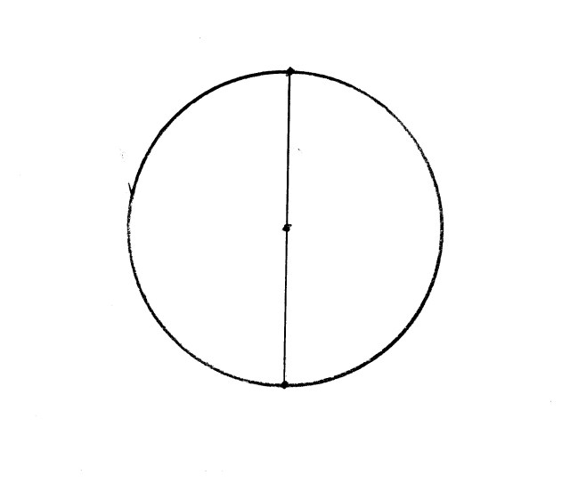
Begin with a circle and mark the focal point. We have actually started with the symbol for Ra, the ancient Egyptian sun god for whom winter solstice was celebrated for thousands of years prior to Judaism – but that may or may not be another story.
Now draw a line vertically through the focal point (i.e. a diameter) and mark its intersection points at the rim.
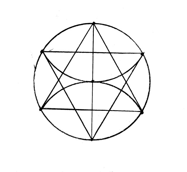
Next set the compass to span from one of the rim intersection points to the focal point and swing an arc through the rim as shown. Mark the arc’s intersection points.
Repeat from the other rim intersection and mark two more rim points.
Connect all the rim points across the circle.
Erase the circle rim, diameter line and interior arcs and you are left with the Star of David.
Now let’s create the Christian cross – also from the intersection of line and circle:
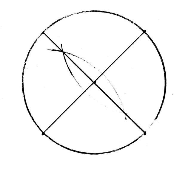
Again we’ll start with a circle (which came to represent the heavens), but this time we’ll draw the diameter line at about a 45° angle.
Construct another diameter line at a right angle to the first. Use the intersecting arcs method (or just fudge it, I won’t tell).
Connect the rim intersection points to create a square (which traditionally represents the four directions, the four seasons and the earth itself).
Now bisect the lower horizontal line and extend the bisection line from the focal point down past the lower rim of the circle.
We’ll set our compass to the span between the rim intersection point and focal point, and swing a second circle. (A second of a pair of circles traditionally represented the Dyad … the reflection, the knowing of the first circle called the Monad (all one/alone).)
When we erase most of the lines we are left with a cross … a symbol of the melding of heaven with earth. Or for the math geeks: a pairing of a diameter line (2) with the non-terminating (i.e. irrational) square root of two.
Note: This geometric construction of the cross is not historical but rather the product of my imagination.
![IMG_2856[1]](https://i0.wp.com/blog.lostartpress.com/wp-content/uploads/2018/01/img_28561.jpg?resize=640%2C853&ssl=1)


![IMG_2802[1]](https://i0.wp.com/blog.lostartpress.com/wp-content/uploads/2017/12/img_28021.jpg?resize=640%2C640&ssl=1)